📚 BERT를 이용한 영화 리뷰 감성분석

BERT를 이용해서 영화 리뷰를 긍정/부정으로 분류하는 감성 분석을 실시한다. 데이터는 IMDB 영화 데이터셋을 아래 링크에서 다운받아서 사용한다.
BERT는 한개 또는 두개의 문장을 입력받지만, BERT의 문장 단위는 실질적으로 사용되는 의미론적인 문장과 다르기 때문에 512개의 토큰까지 하나의 문장으로 간주해서 입력할 수 있다.
✅ 특성 기반 방법 (Feature Based ) vs 미세 조정 방법 (Fine Tuning)
감성 분류는 크게 두 가지 방식으로 접근할 수 있다.
📌1. 특정 기반 방식 : Feature Based
사전학습 모델을 이용해서 각 문서(리뷰)의 특성을 저차원 벡터로 추출하고, 이를 추가적인 분류 모델의 입력값으로 사용해서 문서의 감성을 분류하는 방식이다.
BERT 에서는 CLS 토큰이 각 영화 리뷰에 대한 정보를 포함하고 있기 때문에 이 벡터의 정보를 활용하고, 추가적으로 로지스틱 회귀 모델을 이용해서 감성을 분류한다. 이 과정에서 사전학습모델이 가진 파라미터를 그대로 사용해서 특성 정보를 추출한다. (새로운 학습 데이터를 위해서 추가 학습 X)
📌 2. 미세 조정 : Fine Tuning
새로운 데이터를 이용해서 사전학습모델의 파라미터를 추가적으로 학습한다. 일부 파라미터만 수정하거나 전체 파라미터를 모두 수정할 수 있다.
✅ Feature Based Approach를 이용한 감성분류
특성 기반 방법은 사전학습모델을 그대로 사용하지만, 여기서는 분류를 위해서 로지스틱 회귀 레이어를 추가한다. 로지스틱 회귀에도 추가적인 파라미터에 있기 때문에, 이 파라미터를 학습하기 위한 데이터가 필요하다.
BERT는 여러 개의 인코더 블록으로 구성되고, 각 인코더는 input vector에 대해서 hidden state vector를 반환한다.
BERT에는 필수 토큰을 포함해서 아래와 같은 형태로 시퀀스가 입력된다.
['[CLS]', 'after', 'stealing', 'money', 'from', 'the', 'bank', 'vault', ',', 'the', 'bank', 'robber', 'was', 'seen', 'fishing', 'on', 'the', 'mississippi', 'river', 'bank', '.', '[SEP]']
입력된 시퀀스의 임베딩 벡터 정보를 구하는 방법은 1. 문장을 구성하는 토큰들의 벡터 정보 이용 / 2. CLS 토큰의 정보 이용 이 있다. 이 분석에서는 2번 방식을 사용한다.
또한, 여러 개의 인코더 블록 중에서 어떤 인콬딩 블록들의 정보를 사용할 것인지를 결정해야 한다. 이는 try&error방식으로 분석자가 결정한다. 여기서는 가장 마지막 인코딩 블록이 출력하는 768 차원의 벡터만 사용한다.
따라서 각 영화의 특징은 768개의 벡터로 나타낼 수 있고, 로지스틱 회귀에는 총 768개의 변수가 입력된다.
또한 이 분석에서는 Hugging Face에서 제공하는 TFBertModel을 사용했다. https://huggingface.co/
📌라이브러리 및 데이터 불러오기
import numpy as np
import pandas as pd
import tensorflow as tf
from transformers import TFBertModel, BertTokenizer
import warnings
warnings.filterwarnings('ignore')

df = pd.read_csv('https://github.com/clairett/pytorch-sentiment-classification/raw/master/data/SST2/train.tsv', delimiter='\t', header=None)

df.head()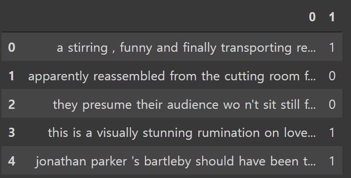
데이터는 영화에 대한 개별 리뷰와 라벨로 구성되어 있다 ( 긍정 : 1 / 부정 : 0 ). 총 행의 수는 6920개이다.

종속변수의 분포는 거의 동일하게 구성되어 있어서, class imbalance 문제는 없음을 알 수 있다.
📌입력 데이터 Tokenize
리뷰 데이터를 BERT 모델에 맞는 형태로 변경해야 한다. 수행해야 하는 작업은 다음과 같다
• 각 영화 리뷰에 [CLS], [SEP] 토큰 추가하기
• 각 리뷰를 BERT 방식으로 토큰화하고, 각 토큰에 ID 부여
• 각 리뷰의 길이를 통일하기 → 길이가 짧은 경우 [PAD] 토큰 추가
• Attenion Mask 부여 : 원래 리뷰의 토큰은 1로, 길이 맞추기 위해서 추가된 토큰은 0 값 부여
이 과정을 BERT에서 제공하는 tokenizer를 사용해서 실시한다.
# 미리 학습된 토크나이저 불러오기
tokenizer = BertTokenizer.from_pretrained('bert-base-uncased')
def encode(sents, tokenizer):
input_ids = [] # 각 문서를 구성하는 토큰의 ID 정보를 저장하는 리스트
attention_masks = [] # 각 문서의 어텐션 마스크 정보를 저장하는 리스트
for text in sents:
tokenized_text = tokenizer.encode_plus(text,
max_length=30, # 문서 길이 30으로 통일
add_special_tokens = True, #[CLS], [SEP] 토큰 추가
pad_to_max_length=True,
# padding_side='right',
return_attention_mask=True)
input_ids.append(tokenized_text['input_ids'])
attention_masks.append(tokenized_text['attention_mask'])
return tf.convert_to_tensor(input_ids, dtype=tf.int32), tf.convert_to_tensor(attention_masks, dtype=tf.int32)tokenized_sents = encode(df[0], tokenizer)tokenizer에서 제공하는 encode_plus() 함수를 사용한다. 여기서는 encode_plus() 함수를 이용해서 encode() 함수를 정의한다. 리뷰와 토크나이저 정보를 입력 받고, 각 리뷰의 토큰ID와 attention mask 정보를 반환한다.
# 첫번째 리뷰의 토큰 ID 정보
tokenized_sents[0][0]

# 첫번째 리뷰의 attention mask
tokenized_sents[1][0]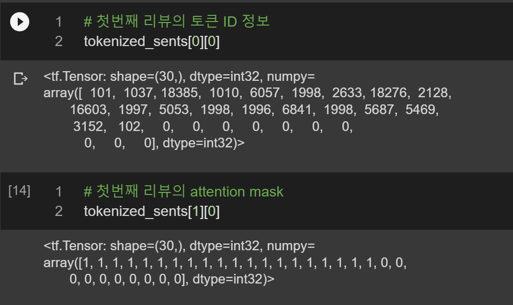
[토큰ID 정보]
첫 번째 리뷰의 토큰 정보에서 101은 [CLS] 토큰을, 102는 [SEP] 토큰을 의미한다. 전체 토큰 길이를 30으로 설정했기 때문에 0인 토큰으로 padding이 실시된 것을 확인할 수 있다.
[attention mask 정보]
패딩을 실시한 토큰인 [PAD]의 경우에는 모두 0으로 표시되고, 원래 존재하던 토큰들은 1로 표시된다.
📌 모델 불러오기 / 학습
model = TFBertModel.from_pretrained('bert-base-uncased', output_hidden_states = True)사전학습 BERT 모델을 불러온다. output_hidden_states = True 로 설정하면 12개의 인코더 블록이 출력하는 hidden states vector 정보를 모두 사용한다.
for layer in model.layers:
    layer.trainable=False
새로 학습을 실시하지 않도록 하기 위해서 layer.trainable=False로 설정한다.
# with tf.device('/GPU:0'):
outputs = model(tokenized_sents[0], attention_mask = tokenized_sents[1])
사전학습 모델을 불러올 때, output_hidden_states = True로 설정할 경우 outputs에는 서로 다른 3개의 원소가 저장되고, 마지막 원소에 모든 인코더 블록에서 출력하는 hidden states 정보가 저장되어 있다.
#마지막 인코더 블록의 정보만 사용
hidden_states[-1]
hidden_states[-1].shape
여기서는 가장 마지막 인코딩 블록의 정보만 사용한다. -1 인덱스를 통해서 가장 마지막 인코딩 블록에 접근할 수 있다. 왼쪽 결과에서 각 리뷰가 30개의 토큰으로 구성되어 있음을 알 수 있다. 여기서는 전체 데이터에서 총 2000개의 리뷰만 선별해서 사용했다. 히든 스테이트 벡터의 크기는 768차원이다.
# CLS 토큰만 선택해서 numpy 배열로 -->독립변수
features = hidden_states[-1][: ,0 , :].numpy()
features.shape

#종속변수
labels = df[1]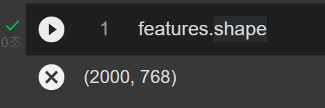
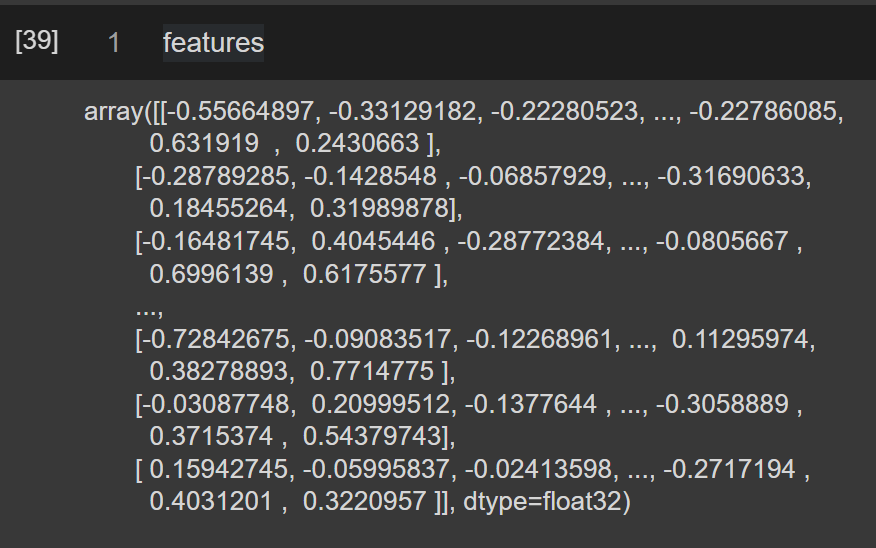
총 30개의 토큰 중에서 첫 번째 토큰인 CLS 토큰의 hidden state 정보만을 사용한다. 따라서 첫 번째 토큰만 선택해서 numpy 배열로 변경한다. 이 배열은 로지스틱 회귀에서 독립변수로 사용된다. 그리고 라벨로 사용할 독립변수도 선정한다.
📌 로지스틱 회귀
일반 머신러닝 모델과 동일한 방식으로 로지스틱 회귀 모델로 분류를 실시한다.
#train/test 나누기
from sklearn.model_selection import train_test_split
train_features, test_features, train_labels, test_labels = train_test_split(features, labels, test_size=0.2, random_state=0)


#로지스틱 회귀 학습
from sklearn.linear_model import LogisticRegression

lr2 = LogisticRegression(C=1, penalty='l2', solver='saga', max_iter=1000)
lr2.fit(train_features, train_labels)
pred_labels = lr2.predict(test_features)


# 정확도 계산
from sklearn.metrics import accuracy_score
from sklearn.metrics import confusion_matrix
from sklearn.metrics import classification_report

#accuracy_score(test_labels, pred_labels)
#confusion_matrix(test_labels, pred_labels)
print(classification_report(test_labels, pred_labels))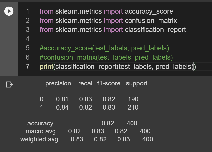
최종적으로 confusion matrix를 통해서 정확도를 확인해보면 0.82 정도이고 전반적으로 precision, recall 점수 또한 준수하다는 것을 확인할 수 있다.
✅ 미세조정 방식 ( Fine Tuning )
미세 조정 방식은 크게 두 가지가 있다.
(1) 기본적인 BERT 모델에 추가적인 신경망 층을 얹어서 사용하기
(2) Huggin Face에서 제공하는 분류를 위한 BertForSequenceClassification 클래스 사용
(2)는 기본적인 BERT 모델에 신경망 층이 추가된 구조를 바로 사용할 수 있다. 여기서는 이 방식으로 분석을 진행한다. 전반적인 방식은 feature based와 유사하지만, 미세 조정 방식은 데이터를 새로 학습해야 하기 때문에 정답 라벨이 있는 데이터를 학습/평가 데이터로 구분해야 한다. 새로 학습을 진행할 때 초기 파라미터는 사전학습 모델의 파라미터가 그대로 사용된다.
📌 라이브러리, 데이터 불러오기
import numpy as np
import pandas as pd
from sklearn.model_selection import train_test_split
import tensorflow as tf
from transformers import TFBertModel, BertTokenizer, TFBertForSequenceClassification
import warnings
warnings.filterwarnings('ignore')

df = pd.read_csv('https://github.com/clairett/pytorch-sentiment-classification/raw/master/data/SST2/train.tsv', delimiter='\t', header=None)

df.head()
동일한 데이터를 이용하여 분석을 진행한다.
# Load pretrained model/tokenizer
tokenizer = BertTokenizer.from_pretrained('bert-base-uncased')
토크나이저를 불러온다
📌 Train/Test 나누기
labels = df[1].values
# labels = torch.tensor(labels)

from sklearn.model_selection import train_test_split
X_train, X_test, y_train, y_test = train_test_split(df[0], labels, random_state=42, test_size=0.2)
📌토큰화
def encode(data, tokenizer):
    input_ids = []
    attention_masks = []
    token_type_ids = []

    for text in data:
        tokenized_text = tokenizer.encode_plus(text,
                                            max_length=50,
                                            add_special_tokens = True,
                                            pad_to_max_length=True,
                                            return_attention_mask=True,
                                              truncation=True)

        input_ids.append(tokenized_text['input_ids'])
        attention_masks.append(tokenized_text['attention_mask'])
        token_type_ids.append(tokenized_text['token_type_ids'])

    return input_ids, attention_masks, token_type_ids
동일하게 encode 함수를 정의해서 토큰화를 실시한다. 여기서는 token_type_ids 정보도 추출하는데, 이는 각 토큰의 문장 임베딩 정보를 포함하고 있다. 여기서는 리뷰가 한개씩 입력되지만, 원래 BERT모델은 두 개의 문장을 입력받기 때문에 동일한 구조로 사용하기 위해서 해당 정보도 추출한다.
#학습데이터 토큰화
train_input_ids, train_attention_masks, train_token_type_ids = encode(X_train, tokenizer)

#테스트데이터 토큰화
test_input_ids, test_attention_masks, test_token_type_ids = encode(X_test, tokenizer)
학습/테스트 데이터에 대해서 각각 토큰화를 실시한다.
📌BERT 모델 입력을 위한 형태로 처리
#딕셔너리 형태로 변환해서 출력
def map_example_to_dict(input_ids, attention_masks, token_type_ids, label):
    return {
      "input_ids": input_ids,
      "token_type_ids": token_type_ids,
      "attention_mask": attention_masks,
      }, label

 #데이터를 BERT에 넣을 수 있는 형태로 변경
def data_encode(input_ids_list, attention_mask_list, token_type_ids_list, label_list):
    return tf.data.Dataset.from_tensor_slices((input_ids_list, attention_mask_list, token_type_ids_list, label_list)).map(map_example_to_dict)
BERT에 입력하기 위해서는 데이터를 딕셔너리 형태로 변경해야 한다.
BATCH_SIZE = 32

#학습 데이터
train_data_encoded = data_encode(train_input_ids, train_attention_masks, train_token_type_ids,y_train).shuffle(10000).batch(BATCH_SIZE)

#평가 데이터
test_data_encoded = data_encode(test_input_ids, test_attention_masks, test_token_type_ids, y_test).batch(BATCH_SIZE)
학습/평가데이터에 대해서 별도로 데이터를 준비한다. 학습 데이터는 shuffle을 이용해서 무작위로 10000개의 데이터를 추출한다.
📌모델 학습
model = TFBertForSequenceClassification.from_pretrained(
    "bert-base-uncased", # Use the 12-layer BERT model, with an uncased vocab.
    num_labels = 2, # The number of output labels--2 for binary classification.
#                     # You can increase this for multi-class tasks.
#     output_attentions = False, # Whether the model returns attentions weights.
#     output_hidden_states = False, # Whether the model returns all hidden-states.
)
TFBertForSequenceClassification 모델을 불러온다.
optimizer = tf.keras.optimizers.Adam(1e-5)
loss = tf.keras.losses.SparseCategoricalCrossentropy(from_logits=True)
metric = tf.keras.metrics.SparseCategoricalAccuracy('accuracy')
model.compile(optimizer=optimizer, loss=loss, metrics=[metric])
NUM_EPOCHS = 10
history = model.fit(train_data_encoded, epochs=NUM_EPOCHS, batch_size=BATCH_SIZE, validation_data=test_data_encoded)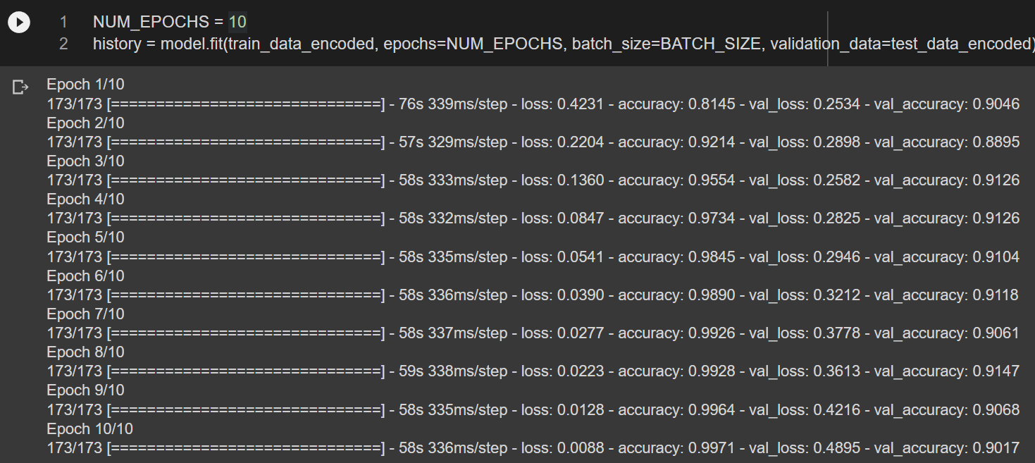
fit()함수를 이용해서 모델 학습을 진행한다. 여기서는 validation set 으로 앞서 정의한 test_data_encoded 를 사용했다. epoch=10인 경우 정확도가 0.9 정도로 향상되었음을 알 수 있다.
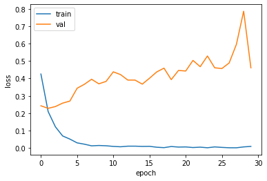
epoch=30으로 학습할 경우 정확도가 0.91로 계산된다.
📌 결과 확인
#loss 확인

import matplotlib.pyplot as plt
plt.plot(history.history['loss'])
plt.plot(history.history['val_loss'])
plt.xlabel('epoch')
plt.ylabel('loss')
plt.legend(['train','val'])
plt.show()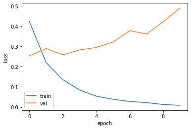
#정확도 확인
import matplotlib.pyplot as plt
plt.plot(history.history['accuracy'])
plt.plot(history.history['val_accuracy'])
plt.xlabel('epoch')
plt.ylabel('accuracy')
plt.legend(['train','val'])
plt.show()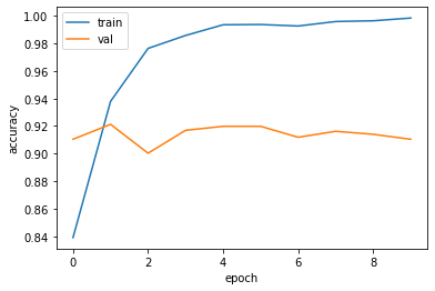
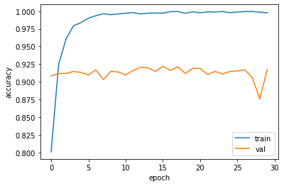
epoch=10인 경우에 대해서 먼저 결과를 확인하고, 추가적으로 epoch=30으로 학습을 진행하였지만 뚜렷한 성능 개선을 확인하지는 못하였다.
📚 Reference
• 연세대학교 디지털사회과학센터(CDSS) 파이썬을 활용한 딥러닝 기초 워크숍, 이상엽 교수님
'머신러닝, 딥러닝 > 딥러닝' 카테고리의 다른 글
| BERT로 한글 영화 리뷰 감성분석 하기 (0) | 2022.02.17 |
|---|---|
| BERT 기본 개념 (0) | 2022.02.13 |
| 오토인코더(Autoencoder), 합성곱 오토인코더(Convolutional Autoencoder) (1) | 2022.01.21 |
| Transfomer 기본 개념 정리 (1) | 2022.01.20 |
| LSTM, Bidirectional LSTM (0) | 2022.01.19 |


댓글