📚 패널 데이터란?

위와 같이 Cross-sectional 데이터와 time-series 데이터의 특징을 둘 다 가지고 있는 데이터를 패널 데이터라고 한다.
→ A panel data set consists of a time series for each cross-sectional member
패널 데이터를 사용함으로써 얻을 수 있는 장점은 다음과 같다.
1. 개인이 가지고 있는 특이성(individual-specific heterogeneity)을 고려할 수 있음
2. 종단/횡단의 두 차원을 결합함으로써 more variation, less collinearity, more degrees of freedom 확보
3. cross sectional 또는 time-series 데이터 각각으로는 파악하기 힘든 영향을 분석할 수 있음
4. Panel data can minimize the effects of aggregation bias.
✅ 예시


unit = 미국 48개 주 / time period = 7년 (1982~1988년)
종속변수 : 교통사고 사망률
독립변수 : 주류세
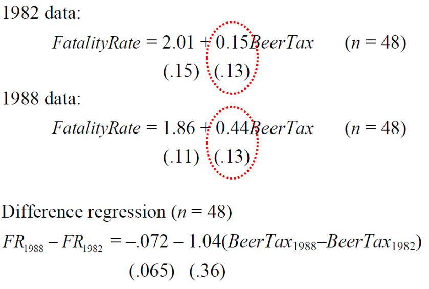
위 예제를 단순히 1988년의 cross sectional 데이터로 분석하면, 주류세가 높을수록 교통사고가 더 많이 발생한다는 결과가 나타난다. (직관과는 반대의 결과)
library(readxl)
tax <- read_excel('Data.xlsx', sheet = 'tax')

coplot(mrall~year|state, type='l', data=tax)
tax$mrall_10k <- tax$mrall*10000

#cross sectional : 단순 회귀
reg_fit_tax <- lm(mrall~beertax+yngdrv, data = tax)
summary(reg_fit_tax)

이는 위 분석에서 통제하지 못한 변수들이 많기 때문이다 → ex. 교통 혼잡도, 음주운전 문화, 자동차의 품질, 도로의 품질
이 변수들을 omitted variable 이라고 부르며 이 문제를 unobserved heterogeneity가 존재한다고 말한다.
✅ Omitted Variable Bias
• In statistics, omitted-variable bias (OVB) occurs when a statistical model leaves out one or more relevant variables. The bias results in the model attributing the effect of the missing variables to the estimated effects of the included variables.
• OVB is the bias that appears in the estimates of parameters in a regression analysis, when the assumed specification is incorrect in that it omits an independent variable that is
(1) a determinant of the dependent variable and
(2) correlated with one or more of the included independent variables.
• OV가 있을 경우 내생성 문제(endogeneity problem)가 있을 가능성이 높다. 여기서 패널 데이터의 특징을 이용하면 OV가 time invariant 할 때 OVB를 제거할 수 있다.
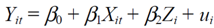
✅ Panel Data Model
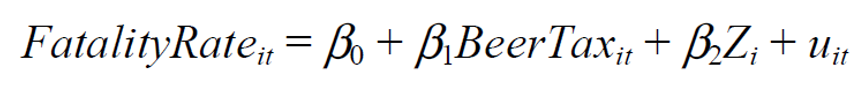
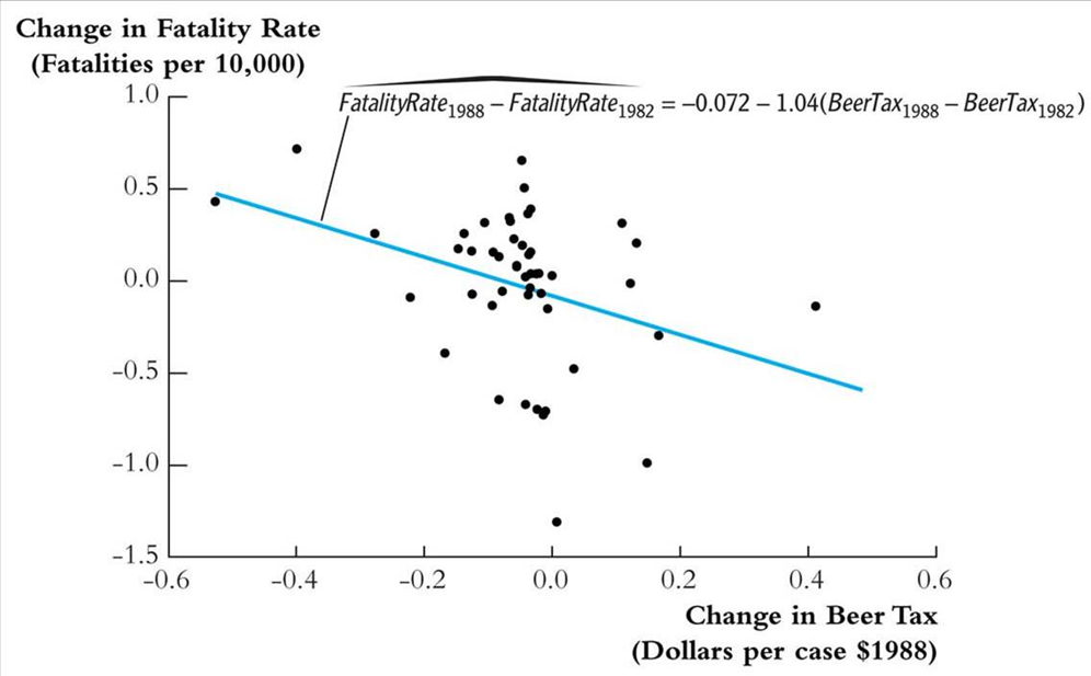
위와 같은 패널데이터 모델에서 uit는 에러 텀, BeerTax의 경우 시간과 state에 따라서 바뀌므로 BeerTaxit로 표시한다.
Zi는 분석기간 동안 time invariant한 특성(예시 : 교통 밀도)을 의미한다.
Zi는 시간에 따라서 변화하지 않기 때문에 1988년 - 1992년 을 빼는 과정을 통해서 Zi의 효과를 완전히 제거할 수 있다. 이렇게 하면 Zi를 직접 관측하지 않고도 차분 식(difference equation)에서 OLS를 실시할 수 있다.
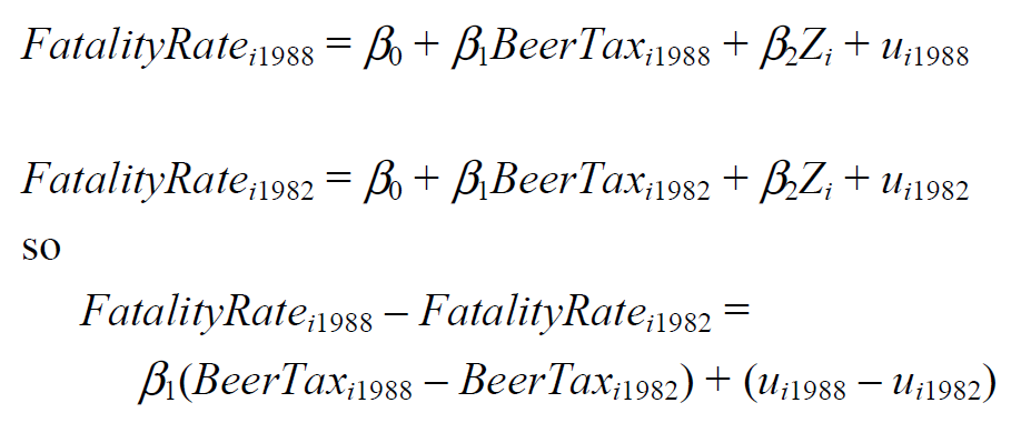
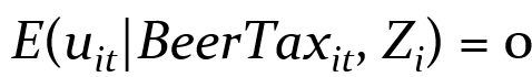
단, 여기서 error term인 uit는 독립변수와 관계가 없어야 한다.
이를 만족할 경우 새로운 error term인 ui(1988) - ui(1982)도 독립변수와 관계가 없게 나타난다.
The new error term, (ui1988 – ui1982), is uncorrelated with either BeerTaxi1988 or BeerTaxi1982.
위 식을 바탕으로 difference regression을 실시하면, 앞선 분석과는 다르게 주류세가 증가할수록 사망률이 감소하는 결과가 나타난다.
📚 Fixed Effects
• 패널데이터 분석에서 분석 단위들(개인, 국가, 회사 등)은 각자 고유한 특성(unobserved heterogeneity)을 가지고 있다. 이러한 변수들은 predictor variable에 영향을 미칠 수도, 미치지 않을 수도 있다. 하지만 데이터 수집 과정에서 이러한 변수를 모두 수집하는 것은 불가능하고, 명시적으로 측정하지 못하는 경우도 많다.
• 따라서 이러한 한계점을 극복하기 위해서 Fixed Effect를 사용한다. FE는 앞서 언급한 time-invariant한 특정을 제거할 수 있어서, 다른 predictor variable로 나타나는 순수한 time-variant effect를 측정할 수 있다.
패널 모델을 추론하는 방법은 크게 세 가지가 있다. (1) LSDV, (2) Wtihin Estimator, (3) First-Difference
✅ 1.LSDV (Least Squares Dummy Variables)
• 패널 그룹의 특징을 이진 더미 변수로 처리하고 회귀분석을 진행하는 방식이다. 이를 LSDV(Least-squares dummy variables)라고 한다. LSDV에는 n-1개의 더미 변수를 포함시켜서 효과를 파악한다. 아래 summary 결과에서 확인할 수 있듯이 모든 state에 대한 더미 변수가 포함된다.
• LSDV는 intercept를 따로 추정하지 않는 모델로, 각각의 더미 변수에 대한 상수항을 구한다. 더미 변수가 많기 때문에 R^2 값은 높게 나타난다.
• 하지만 추정해야 하는 파라미터가 너무 많아서 과적합이 이루어지거나, 자유도 감소 문제가 발생한다. 따라서 패널 그룹의 수가 적고, 패널 그룹 간의 특성 차이가 중요한 경우에 사용한다.
#LSDV
reg_lsdv_tax <- lm(mrall_10k ~ beertax + yngdrv + state -1, data = tax)
summary(reg_lsdv_tax)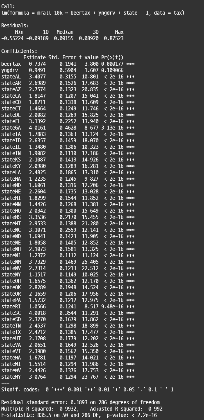
• 반면 FE 모델은 더미변수를 사용하지 않고, within estimation 방식으로 개별 유닛의 그룹의 평균으로부터의 편차를 이용한다. Within Estimator와 LSDV는 결과는 동일하지만 전자가 더 간단하다.
(Unlike LSDV, the “within” estimation does not need dummy variables, but it uses deviations from group (or time period) means. That is, “within” estimation uses variation within each individual or entity instead of a large number of dummies. Within estimator and LSDV estimator are equivalent)
✅ 2. Within Estimator
• 패널 그룹에서 시간에 걸친 평균값을 우선 계산하고, 원래 모형에서 평균값을 제거한
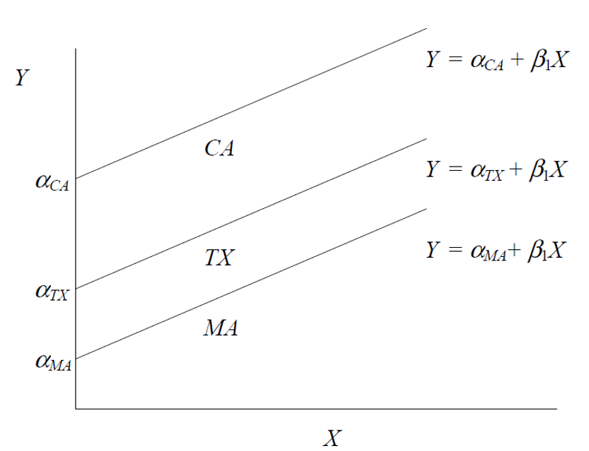
• 위의 데이터에서 만약 state가 3개만(CA, TX, MA)만 존재한다고 했을 때, FE 모델을 시각적으로 표현하면 아래와 같다.
observation N과 time period T에 대한 linear unobserved effects model 은 다음과 같이 작성할 수 있다.

여기서 αi 는state fixed effect이고 state i 끼리는 동일한 값을 가진다. FE 모델에서는 αi를

뺀 식에서 β를 within estormator 또는 FE estimator라고 부른다.
• FE모델을 돌릴 때에는 index 파라미터에 unit of analysis와 time period에 해당하는 변수를 지정한다. model 파라미터는 within으로 설정한다. 분석 결과표를 살펴보면 LSDV와 동일함을 알 수 있다.
• LSDV에 비해서 R^2 값은 작게 나타난다. 일반적으로 FE 모델과 같이 차이를 설명하는 모델은 R^2 값이 낮은 경우가 많다.
#FE model
library(plm)
fixed_w <- plm(mrall_10k~beertax+yngdrv, index = c('state','year'), data = tax, model='within')
summary(fixed_w)
📚 Two-way Fixed Effects
• unit fixed effect 뿐만 아니라 time fixed effect를 고려하는 모델을 two-way fixed effect 모델이라고 한다.

• 주어진 time period에 대해서 T-1 더미 변수를 추가함으로써 time fixed effect를 더한다. 예를 들어 7년 치 데이터가 있고 time period가 1년 단위이면 6개의 시간 변수를 추가해야 한다.
• 독립변수에 년도 변수를 추가한다. 분석 결과를 살펴보면 시간 효과가 반영되었기 때문에 BeerTax 변수의 effect size가 -0.633으로 감소하고, significance도 줄어든 것을 알 수 있다.
• 변수를 추가했으므로 R^2 값은 증가했다. 추가한 변수가 설명력을 제공하기 때문에 BeerTax와 yngdrv의 계수 값은 감소했다.
#Two-way FE model
#year는 numeric 변수이기 때문에 factor로 변경해야 함
fixed_w2 <- plm(mrall_10k~beertax+yngdrv+factor(year), index=c('state','year'), data=tax, model='within')
summary(fixed_w2)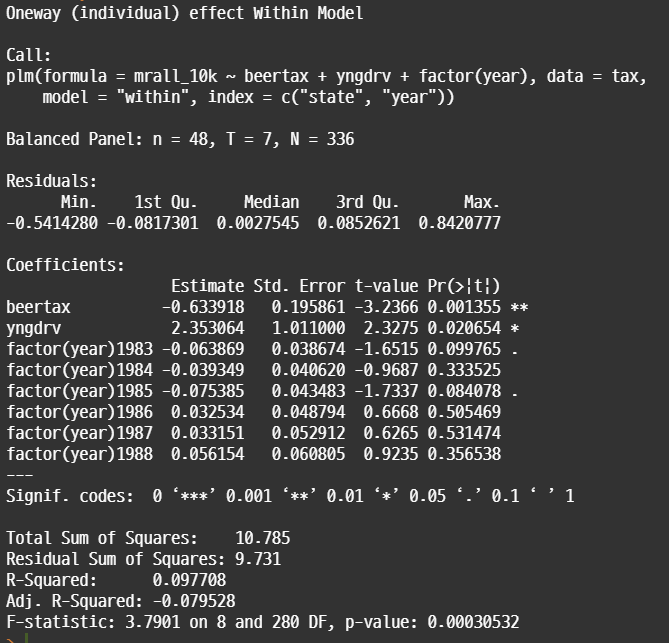
📚 Random Effect
• Individual specific effect에 대한 가정 사항으로는 fixed effect와 random effect가 있다.
The random effects assumption is that the individual-specific effects are uncorrelated with the independent variables.
•If the random effects assumption holds, the random effects estimator is more efficient than the fixed effects estimator. Furthermore, the random effects model allow to estimate the effects of time-variant variables.
• However, if this assumption does not hold, the random effects estimator is not “consistent.”
• The Hausman test is often used to discriminate between the fixed and the random effects models.
• The Hausman test (sometimes also called Durbin--Wu--Hausman test) is based on the difference of the vectors of coefficients of two different models.
• In any case, it is very difficult to justify the use of random effects in academic work
• The αi’s are random variables with the same variance.
• The value αi is specific for individual i.
• The α’s of different individuals are independent, have a mean of zero, and their distribution is assumed to be not too far away from normality.
• The overall mean is captured in β0.
random <- plm(mrall_10k ~ beertax + yngdrv, index=c("state", "year"), data=tax, model="random")
summary(random)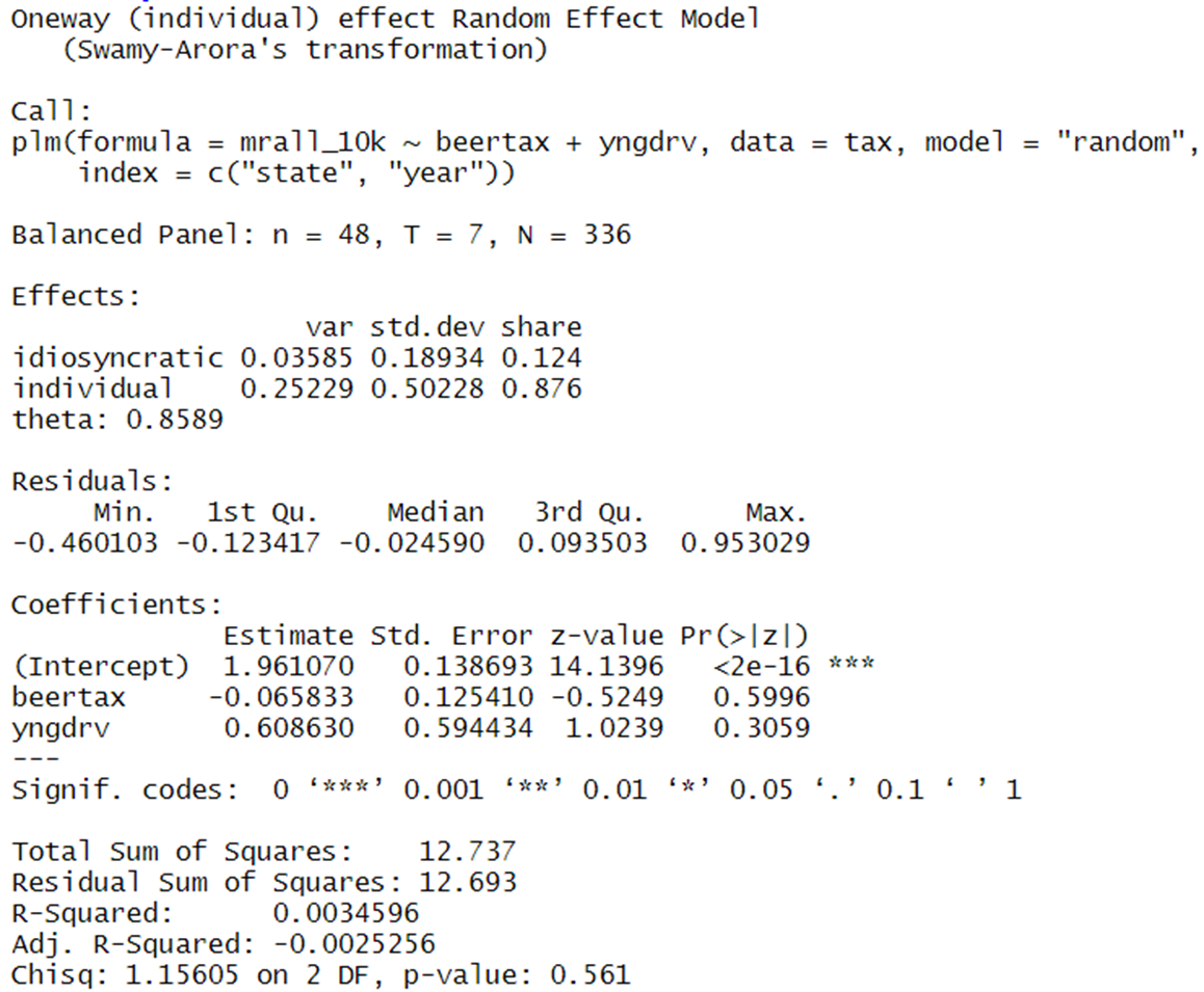
#하우스만 테스트
phtest(fixed_w, random)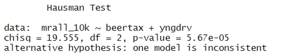
위 결과에서 p-value가 유의한 수준으로 나타나면 fixed effect 모델을 사용해야 함.
📚 Reference
•연세대학교 경영대학, Business Analytics, 김승현 교수
'데이터 분석 > 인과 추론' 카테고리의 다른 글
| [R] Plm vs lm 모델의 R square 값 차이 (0) | 2022.10.02 |
|---|---|
| 도구변수(Instrumental Variable)와 2SLS 분석 (0) | 2022.09.17 |
| Fixed Effect vs Random Effect (1) | 2022.07.03 |
| Difference-in-Differences (이중차분법) (2) | 2022.06.27 |
| DID와 Synthetic Control 비교 (0) | 2022.06.27 |


댓글